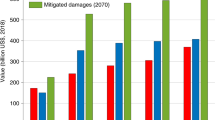
As natural disasters grow in frequency and intensity with climate change, limiting the populations and properties in harm’s way will be key to adaptation. This study evaluates one approach to discouraging development in risky areas—eliminating public incentives for development, such as infrastructure investments, disaster assistance and federal flood insurance. Using machine learning and matching techniques, we examine the Coastal Barrier Resources System (CBRS), a set of lands where these federal incentives have been removed. We find that the policy leads to lower development densities inside designated areas, increases development in neighbouring areas, reduces flood damages and alters local demographics. Our results suggest that the CBRS generates substantial savings for the federal government by reducing flood claims in the National Flood Insurance Program, while increasing the property tax base in coastal counties.
Limiting exposure to climate risks is an important aspect of adaptation to climate change, particularly in coastal areas. As sea levels rise, tidal flooding worsens, and coastal storms become more frequent and severe, limiting the number of people and properties in harm’s way will be key to managing climate damages.
In the United States, state and local governments are primarily responsible for land-use and zoning decisions, but federal policies also play important roles in shaping development. Federal investments in roads, utilities and other infrastructure lay the groundwork for population growth. Other government programmes, such as the National Flood Insurance Program (NFIP), which offers flood insurance at subsidized rates in most locations, and disaster assistance programmes, which provide funding for disaster recovery, also affect location decisions. By partially shifting disaster costs from property owners to the government, these programmes reduce the financial disincentives to development in risky areas.
Whether withdrawing some of these financial incentives would curb development, lower the costs of disasters and help communities prepare for climate change is unclear. Many factors affect development decisions and federal incentives are only some of the factors at play. Empirical research into this question is limited because few policy experiments exist where a clear comparison can be made of ‘treatment’ settings, where incentives for development have been removed, and ‘control’ settings, similar areas where such incentives remain.
One such experiment does exist, however. The 1982 Coastal Barrier Resources Act (CBRA) designated certain areas along the Atlantic and Gulf coasts as a Coastal Barrier Resources System (CBRS). In these areas, most new federal expenditures and financial assistance are prohibited. This includes the prohibition of federal funding for new infrastructure, disaster relief and flood insurance through the NFIP, among others. The law intends to transfer the full cost of private development in these areas from taxpayers to property owners. Besides removing federal incentives, CBRS designations do not otherwise prohibit development. Because the policy is both less restrictive and less costly than most land-use regulations, it may offer an attractive option for managing development in areas at high risk of natural disasters and climate change.
In this study, we leverage the CBRA to study the long-term economic impacts of removing federal incentives in high-risk areas and assess its efficacy as a land conservation and climate adaptation strategy. We not only ask how effective the CBRA has been at discouraging development within designated areas, but also assess the spillover effects of the policy on neighbouring areas.
A recent study employed a spatial regression discontinuity design to compare long-term changes in development densities between CBRS units and areas just outside their boundaries in five states 1 (an update of the authors’ earlier study that used cross-sectional data and an ordinary least squares regression design 2 ). The authors find lower development rates by more than 75% in CBRS areas. However, the regression discontinuity approach, which uses neighbouring areas for comparison with the CBRS, is not appropriate if the CBRS boundaries are based on development levels (Extended Data Fig. 1) and does not allow for the estimation of spillover effects, which our results show are important. Our study provides a comprehensive assessment of the policy’s impact on flood damages, property markets and development, sociodemographic outcomes, and local government finances.
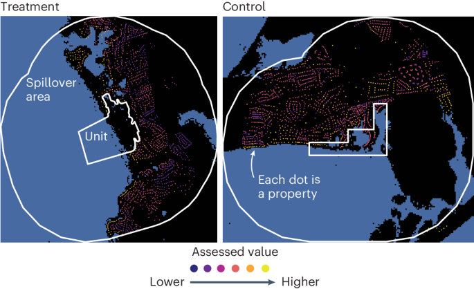
We develop an alternative method for estimating the causal effects of CBRS designations. We construct a control group to compare with the CBRS treatment group using a spatial machine learning technique known as regionalization in combination with a synthetic controls research design. This procedure allows us to mimic the process by which natural resource planners determined CBRS boundaries based on geomorphic and development features (Extended Data Fig. 2), thus identifying a set of coastal areas that could have been selected for CBRS designation in 1982 but were not. To illustrate our approach, we show one example of a CBRS treatment area and constructed control area, overlaid with parcel-level data on the value of properties (Fig. 1).
Our analysis addresses several open questions about land-based climate adaptation. First, it has long been suggested that federal incentives play a role in encouraging development in risky areas 3 , yet quantitative research on this question is limited 4,5,6,7,8 . We evaluate whether the removal of these incentives on coastal lands has been a cost-effective adaptation strategy. Second, by examining the spillover effects of the policy on surrounding lands, we provide estimates of how natural infrastructure affects coastal property values and flood damages, adding to a large literature on the hazard protection and amenity value of natural lands 9,10,11,12,13,14,15,16,17,18,19 . Third, our analysis sheds new light on how removing federal incentives affects local government finances by providing the first estimates of how the CBRA affects property tax revenues. Finally, we show that CBRS designations led to demographic changes, adding to the literature on residential sorting behaviours in response to environmental conditions and land-use regulations 20,21,22,23,24,25,26,27,28,29 .
We measure the effects of removing federal financial incentives for development by comparing outcomes in CBRS units and control areas today. This approach relies on finding control areas that were statistically indistinguishable from treatment areas at the time of designation in 1982, while measuring divergence in outcomes over the four decades since, based on treatment status (Methods).
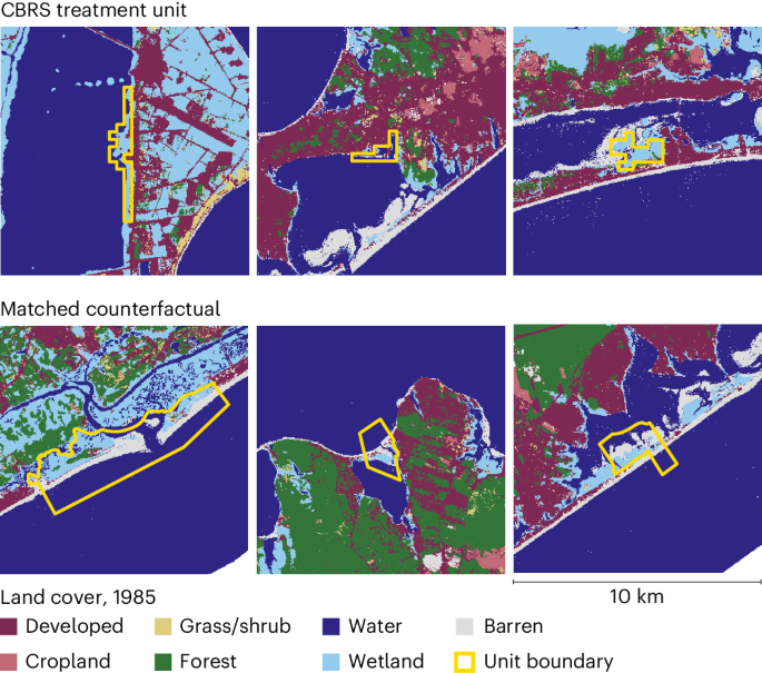
Our spatial machine learning and matching procedure identifies a set of control regions that closely resemble CBRS treatment areas before the policy is implemented (Table 1, Extended Data Table 1 and Extended Data Fig. 3). Treatment and control areas share common pre-trends in development densities (both inside the designated units and in spillover areas) and are balanced across a wide array of pre-treatment observable characteristics, including measures of land cover, elevation, infrastructure density, proximity to urban centres, income and flood risk. To illustrate the output of our procedure, we plot examples of treatment and control units (Fig. 2) and map their geographic distribution (Extended Data Fig. 4).
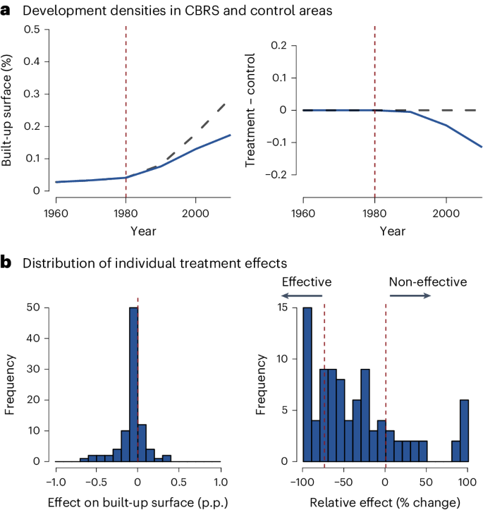
We find that the CBRS has been effective at curbing development within designated areas (Table 2). CBRS designations see 0.12 percentage points (p.p.) less built-up surface area (the percent of land covered by building footprints), a 41% reduction relative to control areas (Fig. 3a). Using an alternative measure of development, we estimate that CBRS units have 0.044, or 83%, fewer buildings per acre than control areas. The magnitude of these effects highlights the central role of federal incentives in shaping development patterns along vulnerable coastlines. Our results pass the standard synthetic control placebo test (Extended Data Fig. 5) and are robust to the use of an alternative research design (Suppmentary Section C).
Local officials may be concerned that by curbing development levels, CBRS designations may adversely affect local property revenues. Using property-level data from Zillow, we do not find evidence of such an effect. We find that CBRS designations increase mean sales prices and total assessed value per acre within designated areas, although the estimates are not statistically significant. Still, the positive effect on prices is consistent with prior evidence that, despite increasing costs for landowners, coastal land-use regulations can increase local property values by restricting supply and generating nature-based amenities 30 . A higher assessed value per acre indicates that the lower development densities are offset by higher average values per property. We find no evidence of systematic differences in the characteristics of properties in CBRS and control areas.
Finally, we examine the impact on local demographics. Because CBRS designations transfer the costs of development and disasters to state and local governments and property owners, the policy may attract homeowners who are more able to bear these costs. Using data from the American Community Survey, we find that CBRS designations increase median household income by US$15,000, or 19%, relative to control areas, and increase the rent-to-income ratio by 2 p.p., or 6%. Thus, CBRS areas tend to attract more affluent residents and have become less affordable for renters. Indeed, the CBRA raises the barrier to entry in designated areas by, for example, necessitating self-insurance against floods 31,32 . Other land-use regulations, such as the California coastal boundary zone, have led to similar demographic shifts 29 .
The occupancy rates within CBRS areas are 14 p.p. lower than those in control areas, suggesting a greater prevalence of second homes or vacation rentals, consistent with policy resulting in greater natural amenities. Finally, CBRS designations changed the racial makeup of residents. While CBRS areas already contained more white people than average coastal areas before designation, we estimate that the policy increased the share of white people by 3% (2.9 p.p.) and reduced the share of Black people by 29% (−1.8 p.p.) relative to the control group.
The efficacy of CBRS designations at detering development may depend on surrounding natural and social systems, including state and local policies. Here, we explore where CBRS designations are more and less effective by estimating unit-specific treatment effects (Methods).
There is a wide distribution of individual treatment effects on built-up surface area (Fig. 3b). Nearly 80% of the unit-level estimates are negative, suggesting that CBRS designations prevent development in most cases. However, the range of estimates is large. Comparing the characteristics of the most and least effective units (Extended Data Table 2), we find that more effective units tend to have lower built-up areas at the time of designation and be larger in size. Natural resource planners ought to consider these characteristics when making new CBRS designations. However, we find no significant differences in pre-treatment land cover, elevation, distance to coast or proximity to urban centres. Additionally, the most effective and least effective units are equally likely to be located on barrier islands or capes, suggesting CBRS designations on these land forms do not have systematically different effects on development from those on the mainland.
The average treatment effect is negative in 10 out of 13 states (Extended Data Table 3), with greater than 50% reductions in built-up area attributable to the policy in Delaware, Georgia, Maine, North Carolina, Rhode Island, South Carolina, Texas and Virginia. We estimate positive average treatment effects in Alabama, Florida and New York. These heterogeneous effects could reflect differences in state and local policies, some of which reinforce CBRS designations by withdrawing local funding in these areas, while others counteract CBRS designations by offering increased subsidies to compensate for the withdrawal of federal incentives. While we find no evidence of systematic differences in pro-environment and pro-development leanings across effective and non-effective units (Extended Data Table 2), prior case studies find the CBRA can be less effective in areas with very high development pressure 33 and powerful growth coalitions 34 .
We next examine whether removing federal subsidies within CBRS designations has an impact on nearby, but untreated, areas. More open space and natural lands in CBRS units might create benefits such as amenity values and flood protective services. These benefits, in turn, might encourage development and demographic changes in nearby areas.
We estimate the impact of CBRS designation on nearby areas as a function of distance to the unit boundary (Fig. 4). We find that removing federal subsidies causes denser development, higher property sales prices and higher assessed values per acre in neighbouring areas. The effect on development densities is increasing in distance from the unit. Within 1,000 m of CBRS units, we estimate an additional 0.03, or 4% more, buildings per acre. Between 1,000 m and 2,000 m, the effect size increases to 0.15 (+20%) and 0.19 (+47%) buildings per acre. The larger spillover effects at greater distances can be explained by the CBRS withdrawing infrastructure investment inside treated units: as transportation and utilities are associated with network effects, we would expect smaller increases in development closer to CBRS boundaries due to limited supply of essential infrastructure.
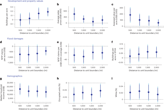
In contrast, average sales prices and assessed values per acre are highest closer to the CBRS units and decline with distance. Properties in the 0–500 m band, for example, sell at a US$377,000 premium, or 77% more than in control areas. Notably, the lower development densities in built structures within CBRS units are more than offset by increased development in neighbouring areas, indicating that the price increases in spillover areas cannot be explained by a supply contraction. Higher property values near CBRS lands are consistent with a large hedonic literature that shows that coastal amenities such as beach access and hazard protection affect real estate markets 13,14,15,16,17,18 .
Higher assessed value per acre in spillover areas results from both denser development (more houses per acre) and higher values per property. Assessed values per acre are US$186,000 higher, or about 50% larger than the control group, in the 0–500 m distance band. The magnitude of this effect decreases gradually with distance.
We next examine the impacts of the CBRS on flood damages in spillover areas. We find economically large and statistically significant negative impacts on overall damages from flooding, as measured by flood insurance claims per acre (Fig. 4d). Annual insurance claims are US$420 to US$760 less per acre (40–64% lower than in control areas). Notably, treatment and control spillover areas have nearly identical shares of land in floodplains (Table 1) and distributions of properties’ distances to the shoreline (Extended Data Fig. 6), suggesting that the differences in flood damages is not caused by geographic differences.
The per-acre measure of flood damages is influenced by development densities in flood zones and flood damages per property. Consistent with the increased development in spillover areas, there are more buildings per acre in high-risk flood zones of CBRS spillover areas as compared with control spillover areas (Fig. 4f). However, flood claims are US$19–27 lower per US$1,000 of coverage in treatment areas (Fig. 4e), representing a 14–25% reduction in flood damages accounting for flood insurance uptake. In other words, the CBRS provides flood protection at the property level. These flood protection services are probably generated by more natural lands inside the units acting as barriers that dissipate and absorb flood waters. Indeed, previous work establishes a link between wetlands and reductions in flood damages 9,10,11,12 .
A back-of-the-envelope calculation shows that the original system of CBRS units generates US$389 million per year in savings for the NFIP. This figure represents approximately 19% of average annual NFIP claims in Atlantic and Gulf coast counties over the period 2009–2021. The original units make up only 0.46% of land areas in these counties. If we assume the CBRS units added later along the Gulf and Atlantic coasts generate similar benefits, the total saving in the current system (excluding the Great Lakes) would be US$930 million per year in annual NFIP claims generated from removing federal development subsidies on only 1% of lands in these counties. This finding complements two existing studies of the savings CBRA generates in federal post-disaster assistance 35,36 .
Finally, we estimate the spillover effect of CBRS designations on demographics (Fig 4g–i). The policy is associated with a large increase in household income (over US$10,000), a decline in the share of occupied housing units (5–8 p.p.), and an increase in the share of white people (1.5–2.5 p.p.). These effects largely mirror the demographic effects of the policy within the designations. Given the above evidence that CBRS lands generate natural amenities and protection services, these results are consistent with past findings on residential sorting in response to environmental amenities 20,37 .
In the spillover areas, unlike in the CBRS, federal flood insurance and disaster aid are still available. Thus the equity implications of the policy are murky. The environmental benefits appear to flow to wealthier households in both the CBRS and spillover areas. But in the CBRS, those households also bear most of the costs of development because federal infrastructure spending, disaster aid and subsidized flood insurance are unavailable. The same is not true in the spillover areas.
We calculate the effect of CBRS designations on property tax revenues by combining our total assessed value estimates in both CBRS units and their spillover areas with current average county property tax rates. We find no evidence of a change in property tax revenues within CBRS designations. However, we find a US$911 million per year increase in revenues in spillover areas. This figure represents 2.5% of total local property tax revenues in Atlantic and Gulf coast states.
Our findings are informative for coastal communities caught between, on one hand, increasing disaster costs, and on the other, the fiscal implications of limiting development. Our calculation suggests that there is not necessarily a hard trade-off between the two objectives. Rather, we show that curbing development in environmentally sensitive areas can increase the property tax base by increasing development densities and property values in nearby locations.
Coastal communities are centres of economic development and home to critical natural resources but face substantial threats from climate change and human development. This paper investigates the efficacy of one policy approach to limiting populations in harm’s way—withdrawing the availability of federal financial assistance in risky areas. We show that, in the case of the CBRA, this approach has been highly effective at limiting development. Moreover, the resulting conservation of natural lands generates environmental services in surrounding communities, increasing property values and reducing flood damages. In combination with analyses of the savings in federal disaster assistance expenditures 35 , our findings provide a comprehensive assessment useful for policymakers.
Methodologically, we develop a new approach for causal inference, using spatial machine learning and matching to construct a comparable control group by mimicking the original CBRA designation process. This approach tackles the central problem of non-random assignment of treatment present in a broad class of place-based policies and could be applied to other settings where it is notoriously difficult to establish causal effects.
Our results indicate that removing federal development incentives can be a cost-effective option for preventing over-development in risky areas while generating co-benefits. Still, programmes like the CBRS are designed to pre-empt development in risky areas, not assist in managed retreat. In areas where strategic relocation of people and capital is deemed necessary, other policy interventions are likely to be required.
Our findings have the potential to inform a number of ongoing policy discussions. The Strengthening Coastal Communities Act (S.5185) would add approximately 292,000 acres to the CBRS. Our estimates could serve as inputs into the cost–benefit analysis of this proposal. More generally, our estimates can inform state- and local-level decisions about zoning practices and government support for infrastructure development and repair in high-risk coastal areas. Notably, our results apply to risky areas beyond just coastlines; a similar approach to managing development could be taken in inland floodplains or in wildfire-prone areas 38 .
Our study has important limitations. First, although we believe our empirical approach represents a step forward, this is ultimately a retrospective, quasi-experimental analysis. Second, our estimates do not capture the full range of benefits and costs associated with CBRS designation. Additional costs may include distortions to the spatial allocation of economic growth 39 , while benefits may include wildlife habitat, water filtration or recreation opportunities. Third, we are not able to observe state and local policies that may either counteract or reinforce CBRS designations. We find heterogeneous treatment effects across states but are unable to attribute those differences to specific policies. Our estimates should therefore be interpreted as the net effect of CBRS designations, inclusive of state and local responses, to the federal policy.
The goal of our empirical strategy is to estimate the causal effect of CBRS designations. The core challenge is identifying a set of appropriate counterfactual units to serve as ‘control’ areas for CBRS ‘treatment’ areas. The CBRA encourages the conservation of biologically rich, underdeveloped and hurricane-prone coastal areas. Therefore, we cannot simply compare our outcomes of interest in CBRS units to those in all other coastal areas; we must identify comparable areas that could have been selected for CBRS designation but were not. We do so using a novel procedure designed to mimic the process by which natural resource planners defined CBRS boundaries. Intuitively, our method for finding counterfactual treatment areas relies on finding locations that are indistinguishable (to the algorithm) from CBRS lands at the time of designation 40,41 .
We first describe the selection process for CBRS designations, as our empirical approach relies on replicating it. The CBRS designation process is described in detail in the 1982 Federal Register and in refs. 42,43 , where the US Fish & Wildlife Service (FWS) establishes a set of ‘definitions and delineation criteria’. CBRS designations were then based upon the application of these criteria to on-the-ground situations.
The first criteria for CBRS designations is that the land should be a ‘coastal barrier’, a class of low coastal land forms that protect landward areas from tidal, wave or wind energies. For the purposes of CBRS designations, the definition of coastal barriers also includes all associated aquatic habitats such as adjacent wetlands, marshes, estuaries, inlets and nearshore waters. In addition to meeting this geological definition, the CBRS requires coastal barriers to be ‘undeveloped’ in order to be included in the system. Specifically, the delineation criteria state that an area should be considered “only if there are few manmade structures on the barrier or any portion thereof and these structures and man’s activities on the barrier do not significantly impede geomorphic and ecological processes” 42 .
According to the Federal Register, Reports to Congress and conversations with programme officers at the FWS, natural resource planners examined US Geological Survey (USGS) topographic maps and aerial photographs to make the original CBRS designations based on just two criteria: (1) adherence to the geologic definition of a coastal barrier, which depends on elevation, land cover and location relative to the shoreline; and (2) development levels.
We now describe our procedure for identifying plausible control areas: areas that could have been selected for CBRS designation in 1982 based on the selection criteria, but were not.
CBRS boundaries do not follow traditional administrative boundaries; they were hand drawn to follow geomorphic and development features 44 . Our first step is to trace out potential counterfactual areas using an automated procedure that closely resembles this process. Importantly, we can observe close proxies for the information the planners had available at the time of designation—aerial photographs and topographic maps (Extended Data Fig. 2). We begin with 300 m resolution gridded data on historical land cover, development levels, elevation and distance to coast. Each cell of the raster represents a distinct observation that will be grouped into a region. We only consider grid cells within 2 km of the coast. We exclude any cell that is 100% water, within a CBRS unit (including both original units designated in 1982 and all units designated since then) or an otherwise protected area, and all grid cells within 2 km of a CBRS unit (to avoid selecting control areas that may be ‘treated’ by spillover effects of CBRS units).
We then apply regionalization to group these pixels into spatially contiguous areas that share similar attributes 45 . Regionalization is one type of clustering—a machine learning technique that sorts observations into groups without any prior idea about what the groups are. Clusters are delineated so that members of a group should be more similar to one another than they are to members of a different group. For example, observations in one group may have consistently high scores on some traits but low scores on others. Regionalization is an application of clustering to spatial data that can be used to provide insights into the geographic structure of complex multivariate spatial data. A ‘region’ is similar to a cluster, in the sense that all members of a region have been grouped together, but a region also describes a clear geographic area. That is, regionalization uses the same logic as standard clustering techniques, but also requires connectivity: two candidates can only be grouped together in the same region if a path exists from one member to another member that never leaves the region 45 (see Supplementary Section B.2 for details).
Regionalization groups all coastal pixels into spatial clusters (‘regions’). We limit our sample to only those regions that would have met the basic requirements for inclusion into the CBRS by conducting a three-to-one propensity score match between the regions and CBRS units based on land cover, development levels and elevation. The algorithm effectively acts as a natural resource planner would have—tracing out low-elevation coastal lands that had high shares of wetlands and beaches (barren), while avoiding highly developed areas. To illustrate the results of this procedure, we show examples of CBRS areas beside matched counterfactuals (Fig. 2). Notably, the adjacent comparisons shown here are not directly used in estimation; we simply provide them to develop the reader’s intuition for how the regionalization algorithm functions. Instead, the matched regions serve as the donor pool for counterfactual units.
Next we apply multi-unit synthetic controls, a technique designed to reduce selection bias in observational studies by weighting the control group to better match the treatment group prior to the intervention 46,47,48,49 . We match on time trends in development densities, both inside the designated units and in spillover areas, for the two decades preceding the policy intervention (1960, 1970 and 1980). We also match on a suite of covariates that we can observe around the time of designation in 1982, including measures of land cover, elevation, infrastructure density, proximity to urban centres, income and flood risk in spillover areas. This allows us to determine a set of weights that, on aggregate, balances pre-trends in development densities and pre-treatment characteristics across CBRS units and the control group. We can then use the synthetic control to estimate what would have happened to the CBRS units if they had not been treated by the policy.
Our empirical strategy requires the CBRS and control areas to have been comparable at the time of designation, while allowing for, and measuring, divergence in outcomes over the four decades since, based on treatment status. We therefore limit our sample to the original set of CBRS units designated in 1982, and all data used in the process of generating counterfactuals comes from as close to this year as possible (and no later than the year 1990). Data sources and processing techniques are described in detail in Supplementary Section B.1.
To illustrate the output of our procedure, we plot the locations of all CBRS and counterfactual units included in our sample (Extended Data Fig. 4). We include control areas in all 18 Atlantic and Gulf Coast states, although four of these states (Maryland, New Hampshire, New Jersey and Virginia) did not have any units in the original CBRS. Because some states had a limited pool of undeveloped coastal areas in 1982, our procedure does not require the distribution of control units to match the distribution of treatment units across states. However, we do balance treatment and control units across three broad regions—the North Atlantic, South Atlantic and Gulf Coast—to avoid making inappropriate comparisons between, for example, coastal areas in Maine and Mississippi.
We assess the success of our procedure for constructing counterfactual areas by comparing the mean characteristics of the CBRS treatment group and synthetic control (Table 1). Encouragingly, our machine learning and matching procedure brings the observable characteristics of CBRS treatment and counterfactual areas into alignment. Column (3) shows that standardized mean difference (SMD) between CBRS and counterfactual areas is at or below 0.1 (the commonly used threshold for accessing balance) across the 18 covariates.
Our approach to identification requires the assumption that not all areas that meet the CBRS delineation criteria were designated as part of the original system in 1982. This assumption is supported by the fact that additional areas have been added to the CBRS over the past 40 years, with the most recent addition proposed in December 2022 50 . According to a 1988 Report to Congress 51 and conversations with programme officers at the FWS, not all eligible areas were designated as part of the original system for two primary reasons. First, USGS quadrangles used in the inventory process did not show sufficient detail to identify all qualifying undeveloped coastal barrier areas. Second, the scientific definition of what qualifies as a ‘coastal barrier’ has evolved over time. We argue that both of these factors are plausibly exogenous to the housing market outcomes we analyse.
One additional concern is that local politics might have affected which areas were designated as part of the CBRS. In particular, if local governments were concerned about the negative impacts of CBRS designation on property tax revenues, they may have objected to CBRS designations in their jurisdiction. Reassuringly, no units were removed from the original proposed set of designations after the public comment period 42 , reflecting limited ability of localities to affect the designation process. Additionally, we empirically test for the presence of this type of selection in two ways. First, we test for differences in local reliance on property tax revenues. Second, we test for differences in the voting records of local members of Congress on environmental issues, as measured by the League of Conservation Voters National Environmental Scorecard, which records the voting records of all members of Congress on major environmental legislation. We find no meaningful differences in either of these measures across treatment and control areas: local reliance on property tax revenues is 35.2% in treatment areas and 35.9% in control areas (P value on difference = 0.61) and environmentally friendly voting records (League of Conservation Voters score) are 57.0 in treatment areas and 56.8 in control areas (P value on difference = 0.96). These results are inconsistent with local politics causing selection away from pro-development and towards pro-environment areas.
It is worth emphasizing the consideration of development levels in the CBRS designation process. The ‘any portion thereof’ language in the definition of an ‘undeveloped’ coastal barrier is key because it means that the statutory definition does not require an entire coastal barrier to be designated as a CBRS unit; the FWS had the authority to include only the portions of the barrier that were underdeveloped. In fact, the boundary was often intentionally placed to exclude developed areas. The Federal Register explains, “the side boundary is placed immediately adjacent to the cluster of structures or the area with a full complement of infrastructure indicating the end of the developed portion of the coastal barrier” 42 . We show an example of this practice for a unit in North Carolina, where developed areas were excluded from the CBRS designation to satisfy the definition of an ‘undeveloped’ coastal barrier (Extended Data Fig. 1a).
The central role of development levels in the delineation process calls into question whether the causal effect of CBRS designation can be identified through a spatial regression discontinuity design, as in ref. 1 . The core assumption of a spatial regression discontinuity—that land located just within and just outside the boundary can be assumed to be similar in all ways except for assignment to treatment—is problematic in this setting because natural resource planners hand-selected CBRS boundaries to avoid already developed areas. To see this, we calculate the mean share of developed land just inside and just outside of CBRS boundaries in 1985 using data from the USGS’s Land Change Monitoring, Assessment, and Projection (LCMAP) product 52 . We find that around the time of designation in 1985, the share of developed land was already 9.6 p.p. (95% confidence interval = 6.5 to 12.8) higher just outside the boundary than just inside the boundary, representing a more than doubling in development levels at the boundary. We define ‘just’ inside and outside using 100 m buffers, following ref. 1 . We find that there is a discrete jump in the share of developed land even as one approaches the boundary (Extended Data Fig. 1b).
Our approach to identification, as described above, explicitly takes into account the consideration of development levels in delineating CBRS boundaries and is designed to be able to recover the spillover effects of the policy on neighbouring areas. Indeed, we find that our procedure does well in replicating the consideration of development levels in drawing CBRS boundaries. Even before the policy was enacted, development levels were 33% higher just outside than just inside CBRS boundaries (within 100 m). We find a similar pattern among our synthetic control areas, where development levels are 24% higher just outside than just inside the boundary.
We examine two sets of outcomes related to the removal of development subsidies: direct effects within CBRS units and spillover effects in neighbouring communities. All outcomes are measured using the most recent data available (2010 onwards) such that we capture the long-term effect of CBRS designation. That is, we compare outcomes today in treatment and control units under the assumption that these two groups were comparable at the time of designation in 1982, and test whether outcomes have diverged over the past four decades based on treatment status.
Direct effects include impacts on development levels, land values, and composition of the housing stock and population. We measure development levels using two different data sources. The first measure is the share of built-up surface area from the HISDAC-US Building Footprint Area (BUFA) database (https://dataverse.harvard.edu/dataverse/hisdacus). Assembled from property assessment records, BUFA is a gridded data product that estimates the sum of building areas at 250 m spatial resolution every 10 years from 1900 to 2010. The key advantage of this dataset is that we can observe the evolution of built-up area over time, including in the decades before CBRS designation. Our second measure of development densities is the number of structures per acre, calculated from Microsoft Maps’ Building Footprint database (https://github.com/microsoft/USBuildingFootprints). This dataset provides approximately 130 million computer-generated building footprints derived from satellite imagery for the entire United States. These data offer higher spatial resolution than HISDAC-US, but only for a single snapshot in time during the post-period.
We measure land values using property sales prices and assessment values from the Zillow Transactions and Assessment Database (ZTRAX) (https://www.zillow.com/research/ztrax/). The ZTRAX dataset also provides information on the composition of the housing stock (for example, lot size, year built, square footage, number of bedrooms). Because outcome data from the ZTRAX Database (property sales prices and characteristics) are incomplete—only about half of treatment and control units have one or more parcels in the database—we calculate a separate set of synthetic control weights for the ZTRAX outcomes (Extended Data Fig. 3 and Extended Data Table 1). Missingness in the ZTRAX database is described in Supplementary Section B.1 and explored at length in ref. 53 .
We evaluate the composition of the population using census block-group-level 5-year estimate (2016–2020) from the American Community Survey. Building footprints and ZTRAX data points are assigned to CBRS units by intersecting the geocoded polygons and points with CBRS boundaries. To calculate census observations for each CBRS area, we aggregate the values from all census block groups that intersect a given CBRS unit using population weights calculated from high-resolution (1 km) gridded population data.
We also examine the effects of CBRS areas on neighbouring communities. To do so, we draw a 2 km buffer around each CBRS unit and counterfactual area. When constructing spillover areas, we exclude any area that is in a current CBRS designation or otherwise protected area. For treatment spillover areas, if a geography falls within the 2 km of multiple CBRS designations, we assign it only to the closest CBRS unit. For counterfactual spillover areas, we exclude any area that is in a spillover area (within 2 km) of a treated unit.
In addition to the outcomes described above, we measure the impact of CBRS designation on flood damages in order to test whether preserving natural lands provides protective services from flooding. We measure flood damages using flood insurance claims from the NFIP, the dominant insurer for flooding in the United States. Notably, homeowners within CBRS areas are not eligible to participate in the NFIP, so we do not look at the direct effect of CBRS designation on NFIP claims. Because flooding is an infrequent event, we average annual flood claims over the years 2009 to 2020. The most granular geographic identifier available in the NFIP claims and policies data at the time of analysis was the property census tract. To estimate the value of NFIP claims in each CBRS spillover area, we aggregate the values from all census tracts that intersect a given spillover area, weighting by the number of buildings located in the Special Flood Hazard Areas designated by the US Federal Emergency Management Agency (the high-flood-risk areas where flood insurance is required for properties with federally backed mortgages). The intuition behind this approach is that the distribution of NFIP policies and claims over geographic space will probably resemble the distribution of structures in areas with high flood risk.
We provide summary statistics for our outcome measures (Supplementary Table B.1). Column 1 shows the mean values in counterfactual areas and column 2 shows the mean values in CBRS units. All means are weighted by the synthetic control weights used in estimation.
Once we have constructed the synthetic control, we estimate the effect of CBRS designations on built-up surface area using a difference-in-differences framework. We use the weighted regression
$$_=\beta (_\times <\mathrmwhere i indexes the CBRS or control area and t indexes the time period. B denotes the percent of land area covered in built-up surface, T is an indicator for whether the area was treated by the CBRS and POST is an indicator equal to one in the post-treatment period. The regression also includes unit-level fixed effects (λi) and a control for whether the unit is located on a barrier island or cape (R). We weight each observation by the synthetic control weight. The error term ε captures unexplained variations. The treatment effect of interest, β, captures any systematic differences in built-up surface area caused by CBRS designation.
For all other outcomes, where outcome measures are not available in the pre-treatment period, we estimate the direct effect of CBRS designation using a simple weighted regression that compares outcomes in treatment areas today with outcomes in control areas today. The estimating equation is
$$where all variables are defined as in equation (1), except here Y corresponds to one of our other outcome variables. The regression is weighted by the synthetic control weights. The treatment effect of interest, β, captures any systematic differences between the outcomes in CBRS and control areas today, under the identifying assumption that these areas would have been comparable in the absence of treatment.
To estimate the spillover effects of CBRS designations on neighbouring communities, we turn to a spatial lag model. This allows us to capture heterogeneity in spillover effects by distance to the unit. The estimating equation is:
$$where the indicator 1[B = b] is equal to one if the observation falls within distance band b relative to the CBRS or counterfactual unit boundary. We use four distance bands, in increments of 500 m, out to a total distance of 2 km. Because we match on built-up surface area in overall spillover areas (not by distance band), we include distance-band level controls for 1985 land cover, flood risk and share protected area (Xi,b). The regression is weighted using the synthetic control weights.
We next explore where CBRS designations are more and less effective by identifying individual counterfactual and treatment effects. This represents a departure from the main analysis, where we pool all treated units and find a set of synthetic control weights that balances the pre-trends in development densities and mean characteristics of treatment and control, on aggregate. We do not employ individual treatment effects in the main analysis because it is not possible to identify an appropriate counterfactual for each individual CBRS unit; some units look very different from all other coastal areas in the United States. For this part of the analysis, we use a paired-down set of matching variables that only includes pre-trends in development densities and pre-treatment land cover, elevation, proximity to urban centres and region. We identify synthetic controls that match well along all of these dimensions for 90 treatments units (55% of the full sample).
We evaluate heterogeneity in the effect of the CBRS on development densities in three ways. First, we report the distribution of treatment effects across the sample of 90 units for which we are able to identify individual treatment effects. Second, we compute average treatment effects by state. Third, we use a classification analysis to compare the average characteristics of the most and least affected units using two-sample t-tests. We define the least affected units as those with a positive estimate of the individual treatment effect and the most affected units as those with treatment effects, measured in relative terms, in the most negative quartile (more than 67% reduction in development densities).
We calculate the approximate impact of CBRS designation on county revenues from property taxes using the equation:
$$where Rc denotes the estimated effect of CBRS designation on property tax revenue in county c. The parameter \(_^\) is our estimated effect of CBRS designation on total assessed value per acre within the CBRS unit and \(_^\) is the estimated effect on assessed value within each distance band b of the CBRS unit. We multiply these estimated effects by the total acreage within the unit, Ac,d, and in each distance band, Ac,b, respectively. Summing these values gives us an estimate of the effect of CBRS designation on total assessed value within the county (the term in parentheses). Notably, this estimate captures the direct effects within CBRS units and the spillover effects on neighbouring properties, both in number and value of developed properties. To estimate the effect on property tax revenue, we then multiply by the county tax rate, tc. This tax rate is derived from the Lincoln Institute of Land Policy Property Tax Database (https://www.lincolninst.edu/data/significant-features-property-tax/access-database/). The nominal tax rate is calculated by averaging municipal and school district taxes and adding them to base county tax rates.
To calculate the impact of CBRS designations on NFIP payouts in spillover areas, we multiply our point estimates of NFIP claims paid per acre (Fig. 4) by distance band with the acres of land in each band. We then sum over all CBRS units to calculate the total impact on NFIP payouts. For savings within the CBRS units, we calculate the average claims per acre across all counterfactual areas and multiply it by CBRS land areas.
In Supplementary Section C, we present results based on overlap weighting under a propensity score matching framework as an alternative approach and robustness check.
All raw data used in this study are publicly available except the property-level information on home values and characteristics from the Zillow Transaction and Assessment Database (ZTRAX), which we accessed through a licence available to researchers. Instructions for accessing raw data are provided in Supplementary Section B.1. The processed datasets are available at https://github.com/hdruckenmiller/cbra. Source data are provided with this paper.
The analysis code is available via GitHub at https://github.com/hdruckenmiller/cbra. The analysis code and scripts are available via Zenodo at https://doi.org/10.5281/zenodo.12199232 (ref. 54 ).
This research was funded by the Lincoln Institute of Land Policy (H.D., Y.L. and M.W.). We thank T. BenDor, P. Mulder, A. Reilly, C. Taylor and D. Wright for helpful comments and suggestions. Property assessment and transaction data were provided by Zillow through the Zillow Transaction and Assessment Dataset (ZTRAX). More information on accessing the data can be found at https://www.zillow.com/research/ztrax. The results and opinions are those of the author(s) and do not reflect the position of Zillow Group.